Convolutional Neural Networks

All of the work we’ve done so far applies to any data set where we can convert the input and outputs to fixed length list of numbers. But we have thrown stout some crucial information.  When we out flatten that image, we lose the fact that there’s meaning in the order of the pixels. And there probably is meaning in the order of the pixels.

Convolutions

Although convolutions have been around for a long time, around 2011 convolutions started being applied to image recognition with huge success.
‍
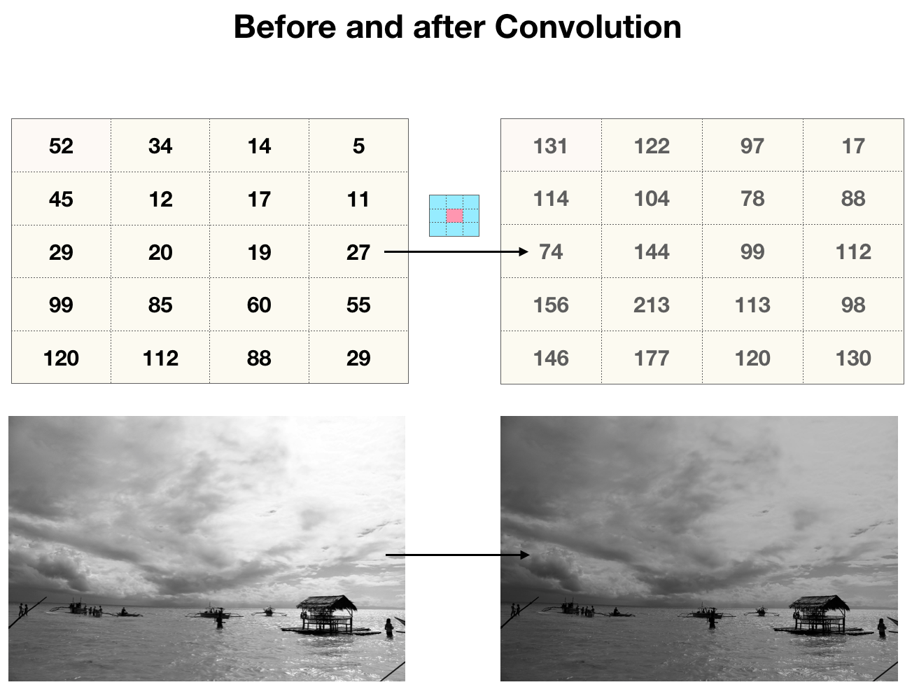
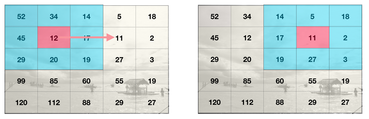
What are convolutions? Convolutions are a way to capture information about the ordering of pixels. The type of convolutions are interested in are 2d discrete convolutions, which act like a weighted sliding sum over an area of pixels. For instance, a 3x3 matrix called a kernel slides across the pixels in an image. At each point, it calculates the weighted sum of the kernels’ values and every pixel in the 3x3 chunk of the image. The sum is then put in the first value of the output image. The kernel then slides over one pixel and repeats the process for every pixel in the image.

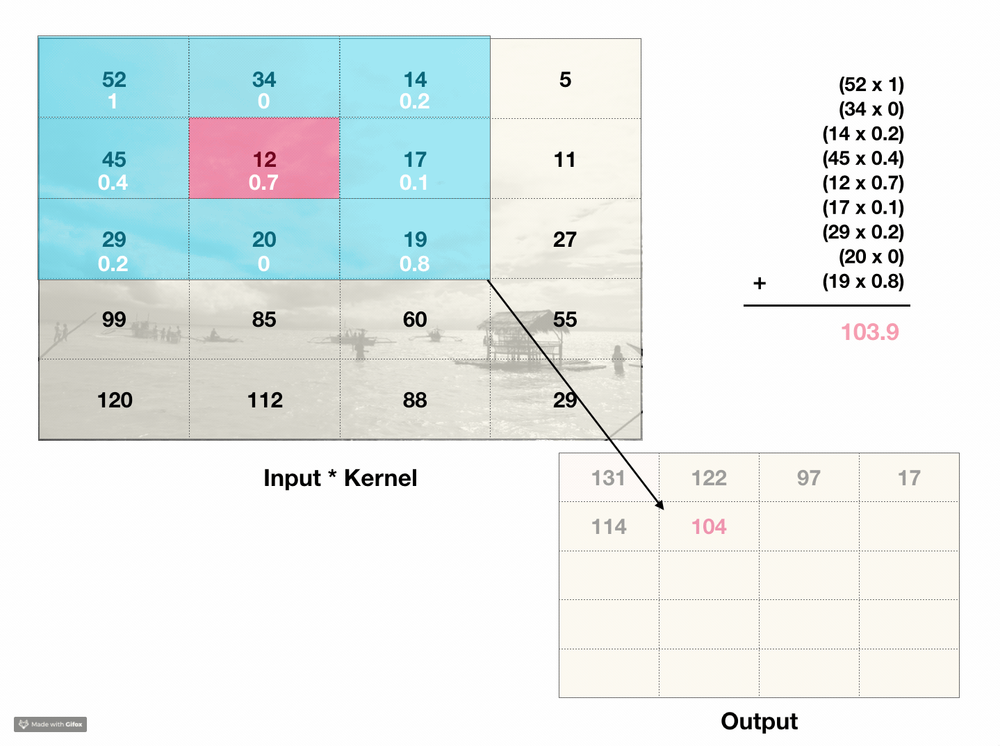
This process incorporates information about a pixels’ neighboring values into its own value. If we compare the original image to the output image, the result looks like a low-budget photoshop filter. For instance, if every value in the kernel was 0.1, the convolution would essentially average over a 3x3 block, so the ‘filter’ in this case would look like a blur.

Color Image Convolutions

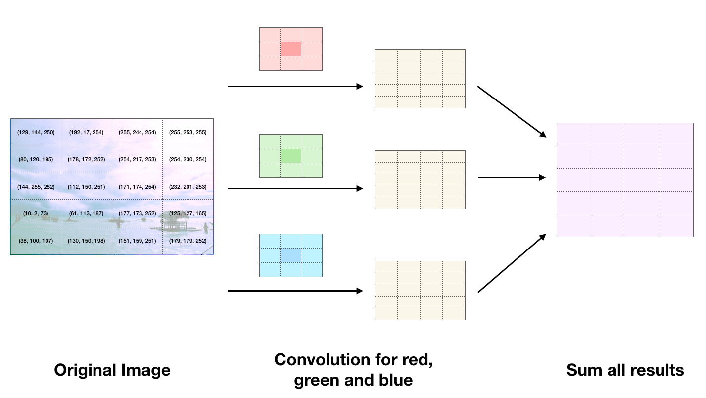
Now that we understand how to perform convolutions on images with single pixel values, an important case to consider is what happens on color images. Pixels in color images have three values - a red, green and blue value. Therefore if we want to run a convolution on a color image we must first break into into red, green and blue components and run one kernel on the red data, one on the green, and one on the blue and sum up all of the results.

Properties of Convolutions

There are several different types of convolutions. Sometimes convolutions take a step of more than one - if each iteration moved by a step of 2 we would say that the convolution had a stride of 2.  

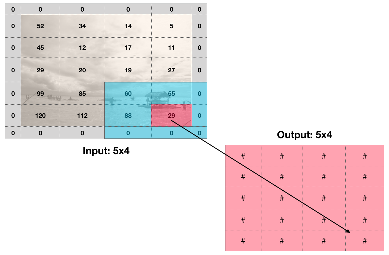
We should also consider how we handle edges.  If we do a 3x3 convolution on an image and we don’t go over the edges, the output image is a little smaller than the input image. This is Keras’ default behavior, but if you want to preserve the image size you can add zeros around the input image, called zero padding.

Pooling

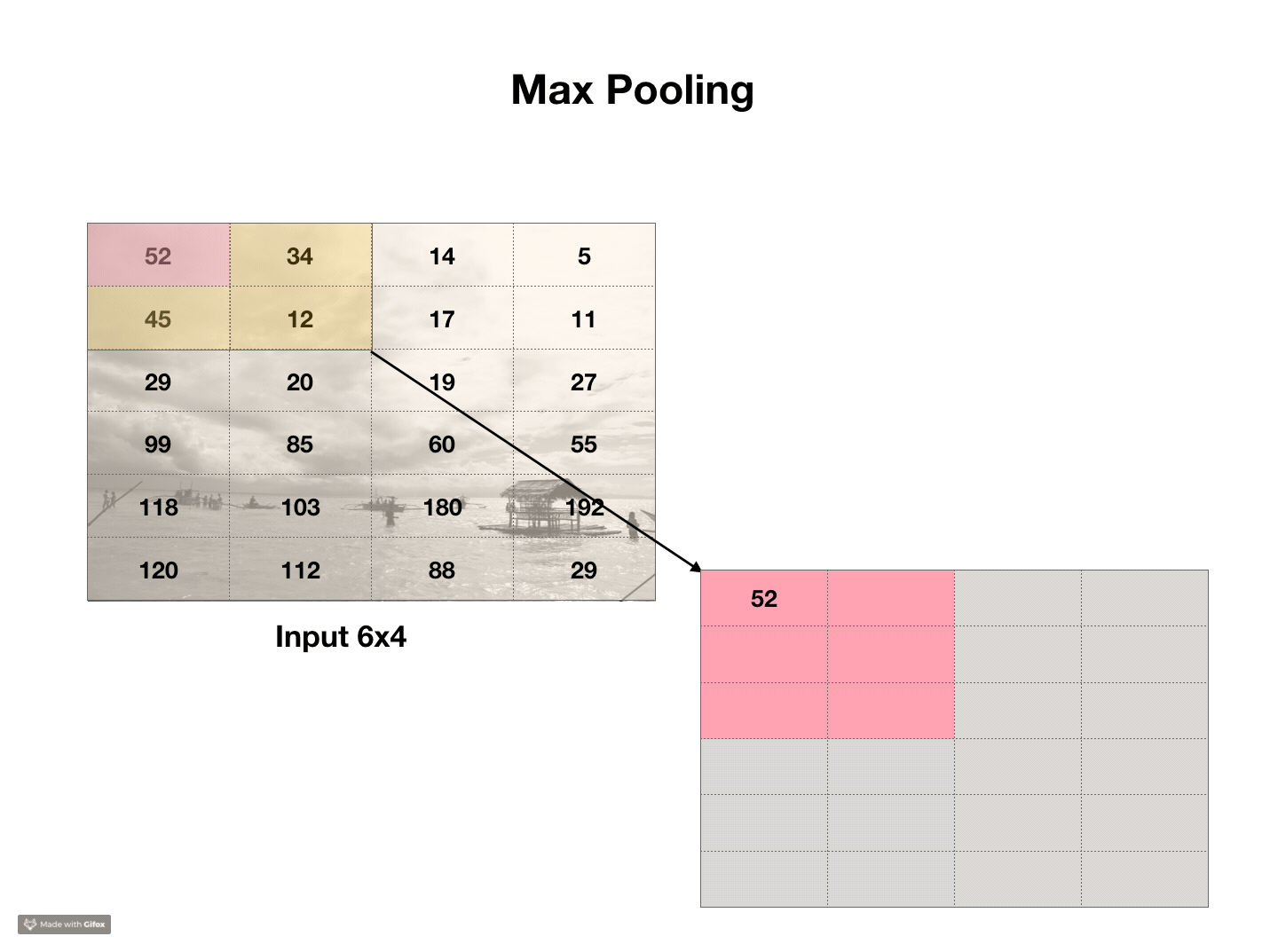
Another, simpler transformation, also very common in neural networks called pooling. If convolutions are a bad photoshop filter, pooling is a bad resizing algorithm. Typically, pooling takes 2x2 regions of an image and chooses the largest value in each region. This is called max pooling. We can do the same with average pooling, where we average over all of the pixels in the 2x2 area. This shrinks the image by a factor of 2, and the area of the image by a factor of 4. The purpose of pooling is to be able to perform convolutions at different scales.

Code

We can now go to the code and see how this all fits together. Open up cnn.py. This code is very similar to where we left off on the multilayer perceptron, with the addition of lines 19 and 20:

// line 19

‍
X_train = X_train.reshape(X_train.shape[0], config.img_width, config.img_height, 1)
X_test = X_test.reshape(X_test.shape[0], config.img_width, config.img_height, 1)

We have to reshape our X data as our image is black and white. Keras expects each input to be a three dimensional image, where the third dimension encodes color. Since our image is grayscale, it does not have this dimension, we have to manually reshape our input and set the color dimension = 1.

The other line that changes in line 29. Until now, we have flattened out our images, but now we are going to do a convolution.

// line 29

‍
model.add(Conv2D(32, (config.first_layer_conv_width, config.first_layer_conv_height), input_shape=(28,28,1), activation='relu'))
model.add(MaxPooling2D(pool_size=(2, 2)))
model.add(Flatten())
model.add(Dense(config.dense_layer_size, activation='relu'))
model.add(Dense(num_classes, activation='softmax'))

This shows that we are doing 32 convolutions in parallel, and we need to learn the weights of each of those parameters. Next, we add a flatten layer that shrinks down the input. Finally, we add a flatten layer, as the next layer is a perceptron (dense layer) and expects a 1 dimensional input.

When we run the model, we see that the number of free parameters are as follows:

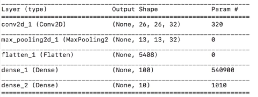
Our model has nearly 1 million free parameters but only 60,000 training data points. What should we be worried about?

The answer is overfitting. And to help reduce overfitting, we always add dropout. Typically we add dropout after layers that have free parameters: in this case, before the first dense layer, and before the second dense layer. We have set dropout = 40%, but it can be anywhere between 20% and 50%. Our code now looks like this:

// line 29

‍
model.add(Conv2D(32, (config.first_layer_conv_width, config.first_layer_conv_height), input_shape=(28,28,1), activation='relu'))
model.add(MaxPooling2D(pool_size=(2, 2)))
model.add(Flatten())
model.add(Dropout(0.4))
model.add(Dense(config.dense_layer_size, activation='relu'))
model.add(Dropout(0.4))
model.add(Dense(num_classes, activation='softmax'))

Now our model has an 98% accuracy. To get to a 99% accuracy, we need to have multiple convolution layers. Why?

The intuition to why we want multiple convolution layers is that after pooling or shrinking, another convolution lets the network learn features over a difference scale on the image. Try adding a few more convolutional layers to your network.

Now you should be getting almost perfect accuracy on this dataset.

Challenge

As another challenge, you might want to try building your own CNN on another dataset. We have already loaded in a similar dataset called fashion MNIST.  It’s 60,000 images but they are of clothes and the categories are "T-shirt/top", "Trouser", "Pullover", "Dress", "Coat", "Sandal", "Shirt", "Sneaker", "Bag" and "Ankle boot".
‍
If you open up fashion.py we have put in some skeleton code that starts off where this whole set of lessons began. Can you apply what you’ve learned to build a fashion classifier on a similar dataset?  

‍